회귀분석 - California_housing 데이터 셋
tf07_california.py
import numpy as np
from keras.models import Sequential
from keras.layers import Dense
from sklearn.model_selection import train_test_split
from sklearn.metrics import r2_score
# from sklearn.datasets import load_boston  # 윤리적 문제로 제공 안 됨
from sklearn.datasets import fetch_california_housing


# 1. 데이터
# datasets = load_boston()
datasets = fetch_california_housing()
x = datasets.data
y = datasets.target

print(datasets.feature_names)
# ['MedInc', 'HouseAge', 'AveRooms', 'AveBedrms', 'Population', 'AveOccup', 'Latitude', 'Longitude']

# print(datasets.DESCR)   # DESCR 세부적으로 보겠다
# 속성 정보:
# MedInc - 그룹의 중위수 소득
# HouseAge - 그룹의 주택 연령 중위수
# AveRooms - 가구당 평균 객실 수
# AveBedrms - 평균 가구당 침실 수
# Population - 모집단 그룹 모집단
# AveOccup - 평균 가구원수
# Latitude - Latitude 그룹 위도
# Longitude - 경도 그룹 경도

print(x.shape)  # (20640, 8)
print(y.shape)  # (20640,)

x_train, x_test, y_train, y_test = train_test_split(
    x, y, train_size=0.7, random_state=100, shuffle=True
)

print(x_train.shape)    # (14447, 8)    # 8(열, column) --> input_dim
print(y_train.shape)    # (14447,)

# 2. 모델구성
model = Sequential()
model.add(Dense(100, input_dim = 8))
model.add(Dense(100))
model.add(Dense(50))
model.add(Dense(20))
model.add(Dense(10))
model.add(Dense(1))     # 주택 가격

# 3. 컴파일, 훈련
model.compile(loss='mse', optimizer='adam')
model.fit(x_train, y_train, epochs=500, batch_size=200)     #batch_size 크면 훈련시간 단축됨

# 4. 평가, 예측
loss = model.evaluate(x_test, y_test)
print('loss : ', loss)

y_predict = model.predict(x_test)

r2 = r2_score(y_test, y_predict)
print('r2스코어 : ', r2)

# loss :  0.6089729070663452
# r2스코어 :  0.5404226100234293
activation 함수 이용
tf08_california_activation.py
# [실습] activation 함수를 사용하여 성능 향상시키기(회귀분석)
# activation='relu'

import numpy as np
from keras.models import Sequential
from keras.layers import Dense
from sklearn.model_selection import train_test_split
from sklearn.metrics import r2_score
# from sklearn.datasets import load_boston  # 윤리적 문제로 제공 안 됨
from sklearn.datasets import fetch_california_housing


# 1. 데이터
# datasets = load_boston()
datasets = fetch_california_housing()
x = datasets.data
y = datasets.target

print(datasets.feature_names)
# ['MedInc', 'HouseAge', 'AveRooms', 'AveBedrms', 'Population', 'AveOccup', 'Latitude', 'Longitude']

# print(datasets.DESCR)   # DESCR 세부적으로 보겠다
# 속성 정보:
# MedInc - 그룹의 중위수 소득
# HouseAge - 그룹의 주택 연령 중위수
# AveRooms - 가구당 평균 객실 수
# AveBedrms - 평균 가구당 침실 수
# Population - 모집단 그룹 모집단
# AveOccup - 평균 가구원수
# Latitude - Latitude 그룹 위도
# Longitude - 경도 그룹 경도

print(x.shape)  # (20640, 8)
print(y.shape)  # (20640,)

x_train, x_test, y_train, y_test = train_test_split(
    x, y, train_size=0.7, random_state=100, shuffle=True
)

print(x_train.shape)    # (14447, 8)    # 8(열, column) - input_dim
print(y_train.shape)    # (14447,)

# 2. 모델구성
model = Sequential()
model.add(Dense(100, activation='linear', input_dim = 8))
model.add(Dense(100, activation='relu'))
model.add(Dense(50, activation='relu'))
model.add(Dense(20, activation='relu'))
model.add(Dense(10, activation='relu'))
model.add(Dense(1, activation='linear'))     # 회귀모델에서 인풋과 아웃풋 활성화함수는 'linear' --> default

# 3. 컴파일, 훈련
model.compile(loss='mse', optimizer='adam')
model.fit(x_train, y_train, epochs=500, batch_size=200)     #batch_size 커야 훈련시간 단축됨

# 4. 평가, 예측
loss = model.evaluate(x_test, y_test)
print('loss : ', loss)

y_predict = model.predict(x_test)

r2 = r2_score(y_test, y_predict)
print('r2스코어 : ', r2)

# result

# activation 을 모두 linear 로 했을 때
# loss :  0.6080942749977112
# r2스코어 :  0.5410859068220331

# loss :  0.4581619203090668
# r2스코어 :  0.6542361534102248
# 모든 히든 레이어에 activation='relu'를 사용하면 성능이 향상됨
다중분류 - iris 데이터 셋
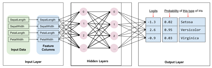
| Feature(특성, 컬럼, 열) |
| sepal length in cm |
| sepal width in cm |
| petal length in cm |
| petal width in cm |
| Class (분류) |
| Iris-Setosa |
| Iris-Versicolour |
| Iris-Virginica |
softmax
tf10_iris_softmax.py
import numpy as np
from keras.models import Sequential
from keras.layers import Dense
from sklearn.model_selection import train_test_split
from sklearn.metrics import accuracy_score
from sklearn.datasets import load_iris
import time

# 1. 데이터
datasets = load_iris()
print(datasets.DESCR)
print(datasets.feature_names)
# ['sepal length (cm)', 'sepal width (cm)', 'petal length (cm)', 'petal width (cm)']

# x = datasets.data
x = datasets['data']
y = datasets.target
print(x.shape, y.shape) # (150, 4) (150,)  --> input_dim : 4 / 다중분류 : Class(분류)

x_train, x_test, y_train, y_test = train_test_split(
    x, y, train_size=0.7, random_state=100, shuffle=True
)
print(x_train.shape, y_train.shape)     # (105, 4) (105,)
print(x_test.shape, y_test.shape)       # (45, 4) (45,)
print(y_test)
# [2 0 2 0 2 2 0 0 2 0 0 2 0 0 2 1 1 1 2 2 2 0 2 0 1 2 1 0 1 2 1 1 2 0 0 1 0
# 1 2 2 0 1 2 2 0]  --> 3가지 분류 (0, 1, 2) => output : 3

# 2. 모델 구성
model = Sequential()
model.add(Dense(100, input_dim=4))
model.add(Dense(50))
model.add(Dense(50))
model.add(Dense(10))
model.add(Dense(3, activation='softmax'))   # 다중 분류

# 3. 컴파일, 훈련
model.compile(loss='sparse_categorical_crossentropy', optimizer='adam',
              metrics=['accuracy'])   # sparse_categorical_crossentropy : one_hot_encoding 하지 않고 가능
start_time = time.time()
model.fit(x_train, y_train, epochs=500, batch_size=100)
end_time = time.time() - start_time
print('걸린 시간 : ', end_time)

# 4. 평가, 예측
loss, acc = model.evaluate(x_test, y_test)
print('loss : ', loss)
print('acc : ', acc)    # acc = 1.0 -> 1로 딱 떨어질 경우 과적합일 확률 높음

# 걸린 시간 :  2.4981889724731445
# loss :  0.041628070175647736
# acc :  0.9777777791023254
one-hot encoding
tf10_iris_onehotencoding.py
import numpy as np
from keras.models import Sequential
from keras.layers import Dense
from sklearn.model_selection import train_test_split
from sklearn.metrics import accuracy_score
from sklearn.datasets import load_iris
import time

# 1. 데이터
datasets = load_iris()
print(datasets.DESCR)
print(datasets.feature_names)
# ['sepal length (cm)', 'sepal width (cm)', 'petal length (cm)', 'petal width (cm)']

# x = datasets.data --> x = datasets['data'] 와 같음
x = datasets['data']
y = datasets.target
print(x.shape, y.shape) # (150, 4) (150,)  --> input_dim : 4 / 다중분류 : Class(분류)

### one hot encoding ###
from keras.utils import to_categorical
y = to_categorical(y)
print(y)
print(y.shape)  # (150, 3)

x_train, x_test, y_train, y_test = train_test_split(
    x, y, train_size=0.7, random_state=100, shuffle=True
)
print(x_train.shape, y_train.shape)     # (105, 4) (105, 3)
print(x_test.shape, y_test.shape)       # (45, 4) (45, 3)
print(y_test)

# 2. 모델 구성
model = Sequential()
model.add(Dense(100, input_dim=4))
model.add(Dense(50))
model.add(Dense(50))
model.add(Dense(10))
model.add(Dense(3, activation='softmax'))   # 다중 분류

# 3. 컴파일, 훈련
model.compile(loss='categorical_crossentropy', optimizer='adam',
              metrics=['accuracy'])   # sparse_categorical_crossentropy : one_hot_encoding 하지 않고 가능
start_time = time.time()
model.fit(x_train, y_train, epochs=500, batch_size=100) # 훈련 시킴
end_time = time.time() - start_time
print('걸린 시간 : ', end_time)

# 4. 평가, 예측
loss, acc = model.evaluate(x_test, y_test)
print('loss : ', loss)
print('acc : ', acc)    # acc 1.0 -> 과적합일 확률 높음

# 걸린 시간 :  2.4981889724731445
# loss :  0.041628070175647736
# acc :  0.9777777791023254

### argmax 로 accuracy score 구하기
y_predict = model.predict(x_test)
y_predict = y_predict.argmax(axis=1)
y_test = y_test.argmax(axis=1)
argmax_acc = accuracy_score(y_test, y_predict)
print('argmax_acc', argmax_acc)
다중분류 - wine 데이터 셋
loss = 'sparse_categorical_crossentropy' 사용하여 분석하기
tf11_wine_softmax.py
# [실습] loss = 'sparse_categorical_crossentropy' 를 사용하여 분석
import numpy as np
from keras.models import Sequential
from keras.layers import Dense
from sklearn.model_selection import train_test_split
from sklearn.metrics import accuracy_score
from sklearn.datasets import load_wine
import time

# 1. 데이터
datasets = load_wine()
print(datasets.DESCR)
print(datasets.feature_names)
# ['alcohol', 'malic_acid', 'ash', 'alcalinity_of_ash', 'magnesium',
#  'total_phenols', 'flavanoids', 'nonflavanoid_phenols', 'proanthocyanins',
#  'color_intensity', 'hue', 'od280/od315_of_diluted_wines', 'proline']


x = datasets['data']
y = datasets.target
print(x.shape, y.shape)

x_train, x_test, y_train, y_test = train_test_split(
    x, y, train_size=0.7, random_state=100, shuffle=True
)
print(x_train.shape, y_train.shape)
print(x_test.shape, y_test.shape)
print(y_test)


# 2. 모델 구성
model = Sequential()
model.add(Dense(100, input_dim=13))
model.add(Dense(50))
model.add(Dense(40))
model.add(Dense(10))
model.add(Dense(3, activation='softmax'))   # 종류 : 0, 1, 2 이므로 3가지

# 3. 컴파일, 훈련
model.compile(loss='sparse_categorical_crossentropy', optimizer='adam',
              metrics=['accuracy'])
start_time = time.time()
model.fit(x_train, y_train, epochs=500, batch_size=100)
end_time = time.time() - start_time
print('걸린 시간 : ', end_time)

# 4. 평가, 예측
loss, acc = model.evaluate(x_test, y_test)
print('loss : ', loss)
print('acc : ', acc)


# 걸린 시간 :  2.5759541988372803
# loss :  0.09535881876945496
# acc :  0.9629629850387573
one-hot encoding 사용하여 분석하기
tf11_wine_onehotencoding.py
# [실습] one hot encoding 을 사용하여 분석
#       (세 가지 방법 중 한 가지 사용)
#       (1) keras.utils 의 to_categorical
#       (2) pandas 의 get_dummies
#       (3) sklearn.preprocessing 의 OneHotEncoder

import numpy as np
from keras.models import Sequential
from keras.layers import Dense
from sklearn.model_selection import train_test_split
from sklearn.metrics import accuracy_score
from sklearn.datasets import load_wine
import time

# 1. 데이터
datasets = load_wine()
print(datasets.DESCR)
print(datasets.feature_names)
# ['alcohol', 'malic_acid', 'ash', 'alcalinity_of_ash', 'magnesium',
#  'total_phenols', 'flavanoids', 'nonflavanoid_phenols', 'proanthocyanins',
#  'color_intensity', 'hue', 'od280/od315_of_diluted_wines', 'proline']

x = datasets['data']
y = datasets.target
print(x.shape, y.shape) # (178, 13) (178,)

### one hot encoding ###
from keras.utils import to_categorical
y = to_categorical(y)
print(y.shape)  # (178, 3)

x_train, x_test, y_train, y_test = train_test_split(
    x, y, train_size=0.7, random_state=13, shuffle=True
)
print(x_train.shape, y_train.shape) # (124, 13) (124, 3)
print(x_test.shape, y_test.shape)   # (54, 13) (54, 3)
print(y_test)


# 2. 모델 구성
model = Sequential()
model.add(Dense(100 ,input_dim=13))
model.add(Dense(50))
model.add(Dense(30))
model.add(Dense(10))
model.add(Dense(3, activation='softmax'))


# 3. 컴파일, 훈련
model.compile(loss='categorical_crossentropy', optimizer='adam',
              metrics=['accuracy'])
start_time = time.time()
model.fit(x_train, y_train, epochs=500, batch_size=100)
end_time = time.time() - start_time
print('걸린 시간 : ', end_time)


# 4. 평가, 예측
loss, acc = model.evaluate(x_test, y_test)
print('loss : ', loss)
print('acc : ', acc)

# 걸린 시간 :  2.516160011291504
# loss :  0.2077403962612152
# acc : 0.9444444179534912'네이버클라우드 > AI' 카테고리의 다른 글
| AI 3일차 (2023-05-10) 인공지능 기초 - Validation split, 과적합(Overfitting)과 Early Stopping (0) | 2023.05.10 |
|---|---|
| AI 3일차 (2023-05-10) 인공지능 기초 - Optimizer (0) | 2023.05.10 |
| AI 2일차 (2023-05-09) 인공지능 기초 - 회귀분석과 분류분석 (0) | 2023.05.09 |
| AI 2일차 (2023-05-09) 인공지능 기초 - 인공지능 기초개념과 훈련 테스트 데이터 셋 (0) | 2023.05.09 |
| AI 1일차 (2023-05-08) 인공지능 기초 - 딥러닝 기본 코드 실습 (4) | 2023.05.08 |


